Doping Windows

1. Overview

Doping windows are used to specify an implant/diffusion doping profile through a window. The vertical profile maybe a Gaussian, a complementary Error function or a user specified profile. Doping windows can also be projected in the upward or downward directions or even in both directions simultaneously. The doping profile of a device is built-up using region doping and horizontal doping windows, which are summed to give a total doping concentration.

2. Usage Instructions

To define a doping window:

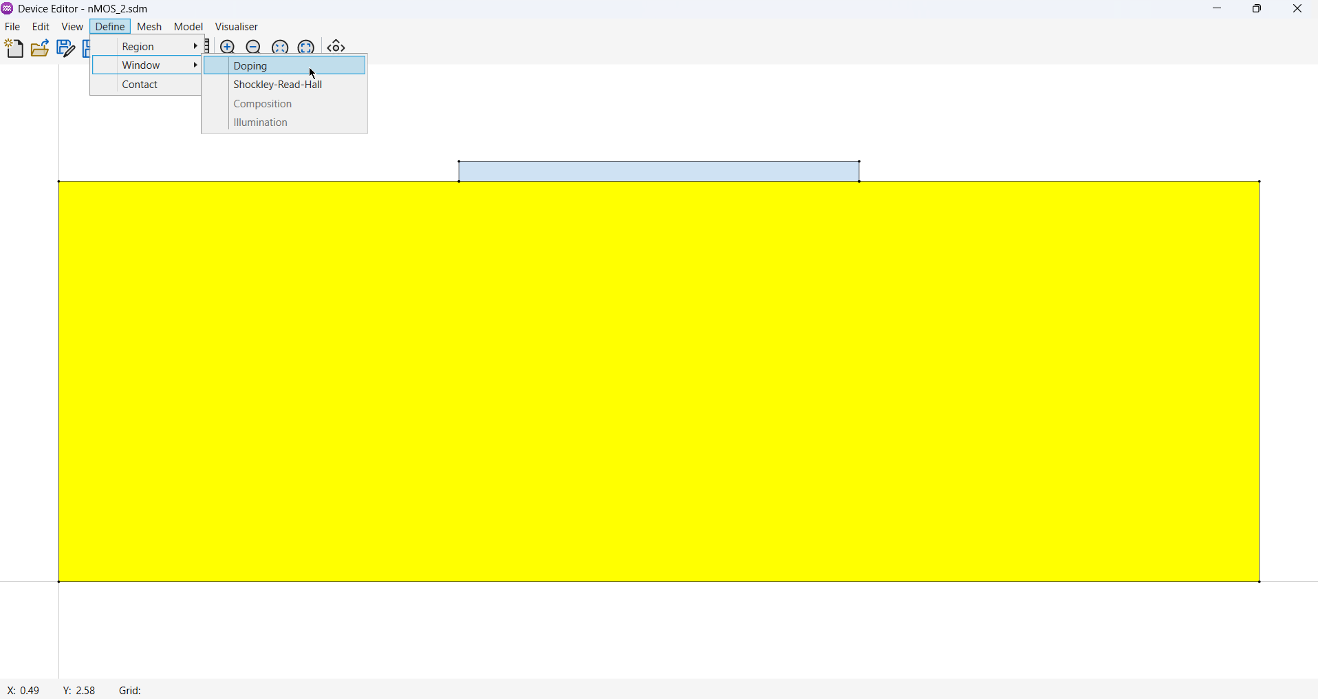
1. From the Menu, select Define -> Window -> Doping.

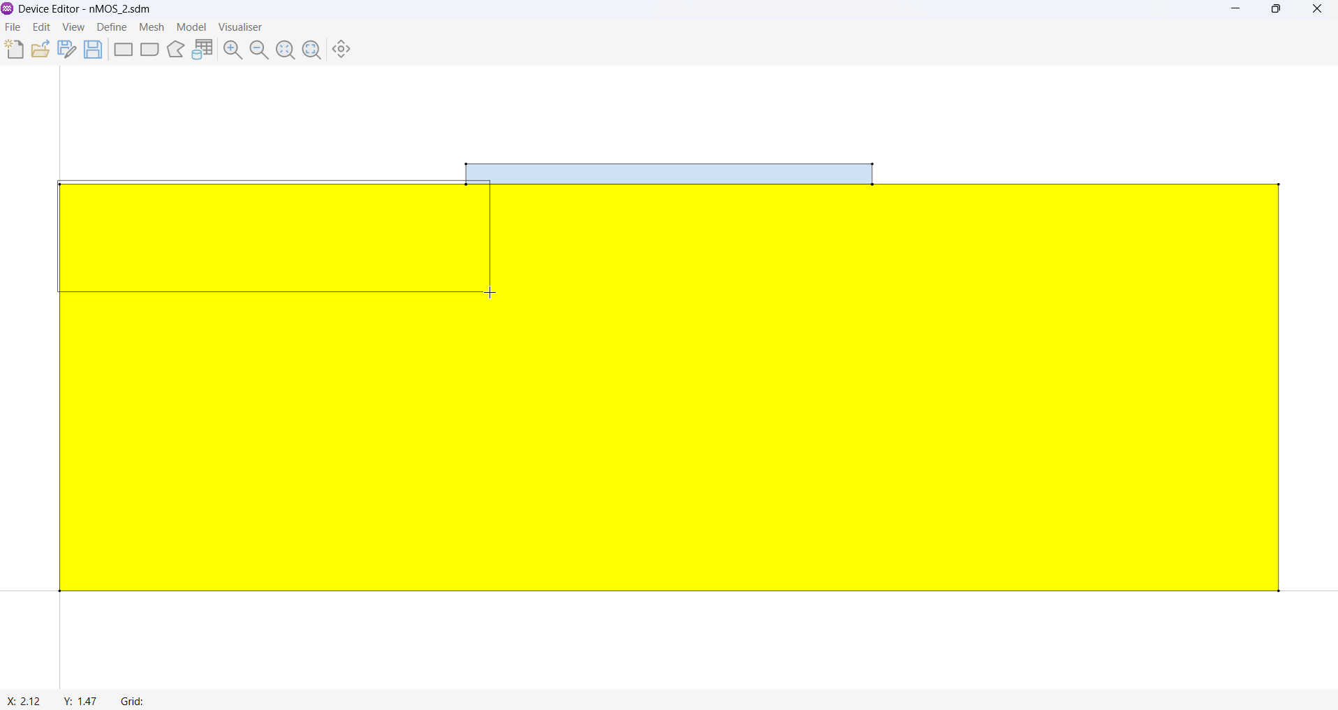
2. Left-click to begin drawing the rectangle and left-click again to finish.

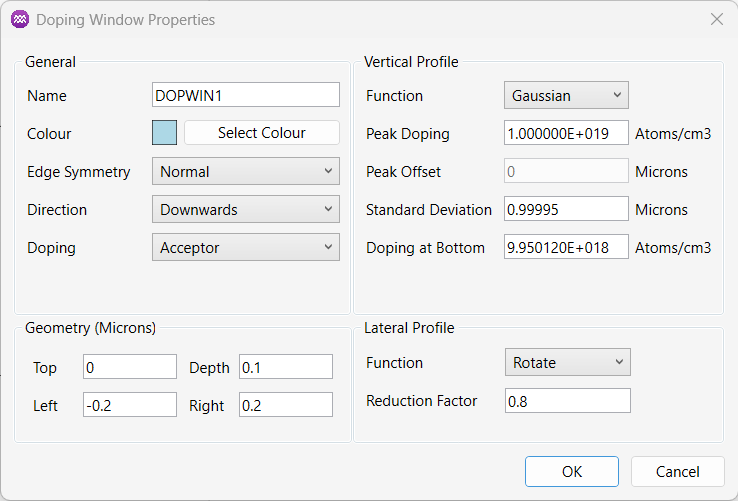
3. Once the window's shape has been defined the doping window's properties dialog box will appear. Use this dialog to set the window's properties.

3. Parameters

3.1. General

Name	Description	Unit
Name	A unique identifier for the window.	-
Colour	Used to define visual colour of the region (Not used in the solver).	-
Edge Symmetry	Used to select the shape of the diffusion. Options: [Normal, Left Symmetric, Right Symmetric or Double Symmetric]	-
Direction	Used to select the direction of the implant. Options: [Upwards, Downwards, Both]	-
Doping	Used to specify the type of doping implant. Options: [Donor, Acceptor]	-

3.2. Geometry

Name	Description	Unit
Surface	Y coordinate of the surface of the window.	μm
Depth	Vertical extent of the window in a direction given by Direction.	μm
Left	X coordinate of the left edge of the window.	μm
Right	X coordinate of the right edge of the window.	μm

3.3. Vertical Profile

Name	Description	Unit
Function	Used to specify the function that controls the scaling of the diffusion in the vertical direction. Options: [Gaussian, erfc, User Defined]	-
Peak Doping	Used to specify the peak doping concentration. For a diffusion implanted in the downwards direction, the peak concentration will occur at the top of the window.	cm-3
Peak Offset	Not used.	μm
Standard Deviation	Used to define the characteristic width of the distribution, determining how rapidly it spreads out from the mean.	μm
Doping at Bottom	Used to specify the doping concentration at the max depth. For a diffusion implanted in the downwards direction, this concentration will occur at the bottom of the window.	cm-3

note

Changing Peak Doping or Doping at Bottom recalculates Standard Deviation. Changing Standard Deviation recalculates Doping at Bottom.

For a user-defined doping profile, the user can specify the data manually or import it from a .csv file. The profile is given as a two-column table: the first column specifies depth (in μm), and the second specifies doping concentration (in cm^-3). The table is applied to the doping window, and linear interpolation is used to compute the doping values at the mesh points beneath the window.

3.4. Lateral Profile

Name	Description	Unit
Function	Used to specify the lateral profile type. Options: [Rotate, Erfc]	-
Reduction Factor	If the Rotate option is chosen then this parameter specifies the lateral reduction factor.	-
Straddle	If the erfc option is chosen then the lateral spread length is specified.	μm

4. Calculation of Total Doping

The applied doping at a given node is defined as:

$$N = N_0 \cdot x_{\text{fact}} \cdot y_{\text{fact}}$$

where:

• $N_0$ is Peak Doping (fixed to 1 for user-defined profiles)
• $x_{\text{fact}}$ is Lateral Scaling Factor
• $y_{\text{fact}}$ is Vertical Scaling Factor

There are two additional considerations which limit the location where doping is applied detailed below.

4.0.1. Edge Symmetry

Before applying any doping, the system verifies whether the node’s X-coordinate falls within the defined window boundaries based on the selected symmetry mode. This check ensures that doping is only applied to nodes positioned within the valid region for the specified symmetry configuration.

• Left-Symmetric: If the node’s X-coordinate is to the left of the window’s left boundary, no doping is applied.
• Right-Symmetric: If the node’s X-coordinate is to the right of the window’s right boundary, no doping is applied.
• Double-Symmetric: If the node’s X-coordinate is outside the left or right boundaries, no doping is applied.
• Normal: All nodes are considered for doping.

4.0.2. Direction

When the doping direction is Upwards or Downwards doping is set to zero in the opposite direction. For example, with Downwards selected, nodes above the surface will have no doping applied.

4.1. Lateral Scaling

4.1.1. Rotation

The lateral rotation adjustment calculates an effective vertical depth ($y_\text{eff}$) for nodes outside the lateral boundaries of the doping window. This is used in place of the vertical depth for the vertical scaling calculation. This creates an elliptical influence region.

• Inside the window (Left $\le X \le$ Right):

  $$y_\text{eff} = \Delta y = |y_{\text{surface}} - y_{\text{node}}|$$

  The effective depth is the absolute vertical distance from the window surface.

• Outside the window:

  $$y_\text{eff} = \sqrt{\frac{(\Delta x)^2}{r^2} + (\Delta y)^2}$$

  where:

  • $\Delta x$ = lateral offset (distance from the nearest window edge)
  • $\Delta y$ = vertical offset (distance from the window surface)
  • $r$ = Reduction Factor, which scales the lateral contribution

This formula increases the perceived depth for nodes that are laterally displaced from the window, reducing their doping influence. A smaller $r$ amplifies the effect of lateral distance, while a larger $r$ minimizes it. Typically, values between 0.5 and 0.8 are used.

note

When the rotate function is used $x_{\text{fact}}$ is always = 1.

4.1.2. Erfc

The lateral factor is calculated using the complementary error function based on the node’s X-coordinate relative to the doping window edges. The formula used to calculate the lateral factor depends on the symmetry setting:

• Normal:

  $$x_{\text{fact}} = \frac{\operatorname{erfc}\left(\frac{x - x_r}{\sigma_l}\right) + \operatorname{erfc}\left(\frac{x_l - x}{\sigma_l}\right)}{2} - 1$$

• Right Symmetric:

  $$x_{\text{fact}} = \frac{\operatorname{erfc}\left(\frac{x_l - x}{\sigma_l}\right)}{2}$$

• Left Symmetric:

  $$x_{\text{fact}} = \frac{\operatorname{erfc}\!\left(\frac{x - x_r}{\sigma_l}\right)}{2}$$

• Double Symmetric:

  $$x_{\text{fact}} = 1.0$$

Where:

• $x$ is the node X coordinate.
• $x_r$, $x_l$ are the window right and left edges respectively.
• $\sigma_l$ is the lateral Straddle.

note

When erfc is used $y_\text{eff}$ is always the actual vertical depth: $|y_{\text{surface}} - y_{\text{node}}|$

4.2. Vertical Scaling

4.2.1. Gaussian

Uses a gaussian function:

$$y{_{\text{fact}}} = \exp \left( - \left( \frac{y_{\text{eff}}}{\sqrt{2} \cdot \sigma_v} \right) ^2 \right)$$

• $y_{\text{eff}}$ is the effective vertical depth.
• $\sigma_v$ is the vertical Standard Deviation.

4.2.2. Erfc

Uses the complementary error function:

$$y_{\text{fact}} = \operatorname{erfc} \left( \frac{y_{\text{eff}}}{\sigma_v} \right)$$

• $y_{\text{eff}}$ is the effective vertical depth.
• $\sigma_v$ is the vertical Standard Deviation.

4.2.3. User Defined

For a user defined profile, $y_{\text{fact}}$ is a linear interpolation of the table of user provided values ($y_i$, $N_i$):

For $y_i \le y \le y_{i+1}$ :

$$y{_{\text{fact}}} = N_i + \frac{(y-y_i)}{(y_{i+1}-y_i)} \cdot (N_{i+1}-N_i)$$

Outside the range of $y_i$ values provided:

$$y{_{\text{fact}}} = 0$$

note

When a user defined vertical profile is used, peak doping ($N_0$) is always 1.